Our methodology
How a report is made
The file goes through the steps below, in order. Each chapter names the method, the settings it runs at, and where it stops being reliable. Read it top to bottom, or skip to the chapter you came for.
1 · Scope and notation
The input is a consumer SNP-array export: one row per marker, carrying an rsID, a chromosome, a position and one or two allele letters. The output is a set of estimates computed against public reference panels. No sequencing is involved, no sample is held, and no genotype is compared against another customer's.
Notation used throughout. A genome contributes a dosage gm ∈ {0, 1, 2} at marker m, the count of alternate alleles, with −1 reserved for a missing call. A reference population k has alternate allele frequency fkm. Mixture proportions are written qk, non-negative and summing to one. Allele-frequency statistics over four populations are written f4(A, B; C, D).
- 01Parse
Vendor and compression determined from file content, never from the filename. - 02Lift
Coordinate build measured by trial liftover, then converted to GRCh38. - 03Resolve strand
Calls placed on the reference forward strand where that is decidable; the rest dropped and counted. - 04Grade
Call rate, marker count, heterozygosity, sex-chromosome coverage. - 05Fit
Supervised admixture, block bootstrap, principal components, regional refit. - 06Compare
Allele sharing against excavated genomes; f-statistic admixture models; archaic counts. - 07Call
Uniparental haplogroups; runs of homozygosity.
Your file is kept and used to build future reference panels. No genetic data reaches a log, a trace or an analytics event — there is a test that proves this and it is part of the build.
2 · Reading a genotype file
Six formats are parsed: 23andMe, AncestryDNA, MyHeritage, FamilyTreeDNA, LivingDNA and VCF, each optionally gzip- or zip-compressed. Compression is detected from magic bytes and format from the first 64 kB of content. Each parser returns a confidence; the highest wins, a result below 0.5 is refused, and two parsers within 0.05 of each other at equal priority raise an ambiguity rather than picking one. MyHeritage and FamilyTreeDNA share their column layout and quoting, so the preamble is the only discriminator and the confidences are graded accordingly.
No-call tokens are enumerated rather than inferred: --, -, 0, 00, N, NN, . and ./.. A half-call such as A- yields no genotype. VCF is excluded from that set, because 0 in a VCF is a haploid reference call and treating it as missing voids every Y and mitochondrial genotype in the file. Multi-allelic VCF rows are skipped.
A no-call that survives as homozygous reference is undetectable downstream and biases every proportion toward whichever reference population the panel is richest in, so missingness is carried as −1 to the estimator rather than imputed at any point.
3 · Determining the coordinate build
Consumer exports are mostly GRCh37, a substantial minority are NCBI36, and the reference panel is GRCh38. A file lifted under the wrong chain has every downstream position wrong, so the build is measured rather than read from the header.
Up to 20,000 of the file's own sites are lifted under each candidate chain and the chain landing the most sites on a real panel position is selected. A chain landing fewer than 100 leaves the build undetermined. Lift success rate cannot be used for this: both chains lift close to 100% of sites, and only landing on the panel separates them.
| File | NCBI36 chain | GRCh37 chain |
|---|---|---|
| hu0257DA | 5 | 3,392 |
| hu011C57 | 3,742 | 4 |
The declared build is not evidence. Across 400 real 23andMe exports, 7.6% are NCBI36 and every one of them declares GRCh37 at full confidence. In a wider corpus, 86 of 245 build-detectable files are NCBI36, some dated as early as 2010, and 119 of 467 declare no build at all.
Only primary chromosome-to-chromosome chains are retained; alternate contigs would map array markers onto haplotypes the panel does not contain. A site falling in a chain gap is dropped and counted rather than passed through at its original coordinate, which would be a silent mixture of two builds.
The measurement above is performed on every submission and is used by the Y-chromosome path. The autosomal normalisation path is currently constructed with the default GRCh37 chain regardless of the measured result, because the measured value is overwritten before the normaliser is built. For an NCBI36 export this produces the failure the measurement exists to prevent. It is recorded here rather than described as working.
4 · Strand resolution
An array may report a call from either strand. Where the observed alleles match the reference pair the call is kept; where their complements match, the call is complemented. Two classes cannot be resolved this way. An A/T site complements to T/A and a C/G site to G/C — the same unordered pair — so the observation is equally consistent with both strands.
Three mechanisms exist for these sites: a per-marker chip strand annotation, a frequency comparison against the reference, and dropping. Only the third is reachable on a submitted file, because neither a strand annotation nor a cohort frequency is available for a single genome. Every strand-ambiguous site is therefore dropped and counted, at an expected rate of 2 to 3% of in-reference sites. The frequency mechanism is used during reference-panel preparation, where a cohort frequency does exist, and is gated at minor allele frequency 0.40 with an agreement tolerance of 0.15; both orientations are tested and the site resolves only when exactly one fits, because the two acceptance windows overlap between MAF 0.35 and 0.40 and a first-fit rule silently swaps alleles inside that band.
A third allele — an observation containing a base that is neither reference, alternate, nor a complement of either — is detectable only at strand-ambiguous sites, since at an A/G site the reference pair and its complement span all four bases. It is recorded separately and does not change the disposition, which stays a mismatch drop.
The panel holds 12,770 markers. How many a given file reaches depends on which array produced it: a genuine 23andMe v5 export in the demo set reaches 10,317 of them. The two are different array design lineages rather than two draws from one distribution.
5 · Quality control and floors
Files are graded A, B, C or rejected on the worst of several independent checks. The grade describes the file.
| Check | Reject below | Grade C | Grade B |
|---|---|---|---|
| Call rate | 0.90 | 0.95 | 0.98 |
| Markers in file | 10,000 | — | — |
| Heterozygosity | <0.15 or >0.45 | — | — |
| Y call rate, if male | 0.30 | — | — |
| X heterozygosity, female | 0.15 | — | — |
Human populations sit near 0.30–0.36 heterozygosity on typical array marker sets, and South Asian samples with substantial endogamy sit legitimately at the low end, so the lower bound is generous and low heterozygosity is treated as informative rather than as a defect. Heterozygosity outside the bounds usually indicates the file is not a single human genome.
Sex is inferred from two independent signals, Y call rate and X heterozygosity. Where they disagree the result is undetermined and no value is asserted.
Three overlap floors apply in sequence: at least 15% of panel markers covered, at least 3,000 markers for the admixture fit, and the same 3,000 for the principal-component projection. On the current panel the absolute floor binds, the fractional one being looser. The floor was re-measured when the panel changed size rather than inherited: the previous value was set against a 91,598-marker panel and would have demanded 78% of this one.
| Overlap | Median | p90 | Worst |
|---|---|---|---|
| 10,000 markers | 1.06 | 4.11 | 19.07 |
| 20,000 markers | 0.58 | 3.40 | 10.43 |
| 40,000 markers | 0.35 | 1.94 | 4.78 |
| 80,000 markers | 0.12 | 0.67 | 2.96 |
Displacement is in percentage points. The largest component never changed at any overlap tested, including 10,000, so the floor protects regional detail rather than the leading estimate. Error declines smoothly with overlap and there is no cliff, so any floor is a decision about tolerable error rather than a threshold found in the data.
6 · The reference panel
Allele frequencies are computed from published reference collections. The count below is the number of individuals each collection contributes to the matrix the frequencies are computed from; a collection held but not fitted against does not appear.
| Collection | Individuals | Licence, as recorded in the project manifest |
|---|---|---|
| Allen Ancient DNA Resource (AADR) v66.p1 — 1240K and Human Origins builds | 9,859 | CC0 1.0 as published for v66.p1, but verify current terms before revenue. |
| 1000 Genomes Project, phase 3 — Omni 2.5M array genotypes | 2,446 | Fort Lauderdale / unrestricted public use |
| Indian tribal + HGDP/SGDP/Illumina-Diversity merged reference panel, NIBMG BMCB2021 (Tagore et al. 2021, BMC Bioinformatics) | 1,416 | Public deposit on NIBMG's own data service (share.nibmg.ac.in, Seafile). |
| India-recruited cohorts, the aggregate tag in our genome index | 1,369 | not recorded |
| Worldwide Affymetrix genotypes (Xing et al. 2010), via the Internet Archive | 687 | UNRESOLVED. |
| Coorg (Kodava) and South Asian reference genotypes, Mukhopadhyay et al. 2025, Zenodo 13913147 | 617 | CC-BY-4.0 as declared on the deposit. |
| GEO series GSE242813, the case arm | 192 | not recorded |
| GEO series GSE242813, the control arm | 180 | not recorded |
| Schizophrenia cases and healthy controls, South India, GEO GSE242813 | 180 | NO LICENCE STATED on the GEO deposit; NCBI states its GEO data carry no restrictions while warning submitters may retain rights (ADR-0030). |
| Coronary artery disease cases/controls, Mumbai (Hinduja), GEO GSE109068 | 150 | NO LICENCE STATED on the GEO deposit; NCBI states its GEO data carry no restrictions while warning submitters may retain rights (ADR-0030). |
| gse33489-metspalu | 141 | not recorded |
| India-recruited genotypes, Estonian Biocentre (Metspalu 2011) | 140 | UNRESOLVED, same posture as ebc-munda. |
| mondal-2016 | 68 | not recorded |
| GEO series GSE93037 | 65 | not recorded |
| Munda and Northeast Indian genotypes, Estonian Biocentre | 26 | UNRESOLVED. |
| assam-2026 | 10 | not recorded |
| Khasi Austroasiatic genotypes, NIBMG (Tagore et al. 2022, Mol Biol Evol) | 8 | Public deposit on NIBMG website. |
| Markers | 12,770, the sites a consumer array and the references share, LD-pruned by physical spacing at 20 kb with a minor allele frequency floor of 0.05 |
|---|---|
| Stage one | 16 continental components |
| Stage two | 103 regional components, fitted only inside a continent carrying at least 5% of the genome |
| Component floor | 25 individuals; 125 of 770 labelled populations clear it |
| Ancient reference | 13,468 excavated genomes indexed, 6,776 present-day, 20,244 in total |
Licences are shown in one line. The full statement for each, with the citation its terms require, is on the attribution page, generated from the same manifest. The individual genomes are listed at every genome hosted.
Where the table reads not recorded, the manifest carries no licence field for that collection. That is a gap in the record rather than a claim that the data is unencumbered.
7 · The component register
A component is a set of reference populations pooled into one allele-frequency vector. The populations listed below are the exact labels pooled, read from the table the panel builder reads, so this page cannot describe a pooling that is no longer run. The colour beside each name is the colour that component is painted in a report.
Each region's territory is drawn from the recorded recruitment localities of its own people: 92 from districts where district boundaries are held, 3 as a smoothed envelope around the localities, and 8 as markers on a locality where the population has no territory to draw. No region is derived from a country or province outline. Construction is described in §19.
All 103 boundaries as a single file: the region atlas. The same map is below, carrying each region's population list.
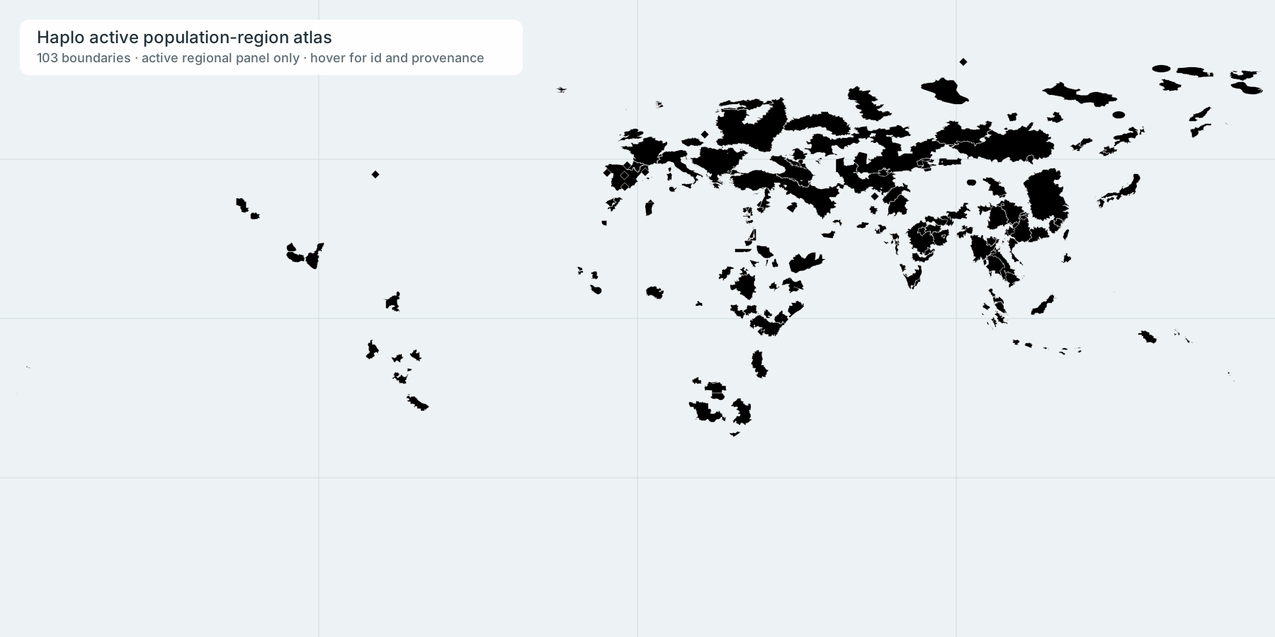
Drag to move. Double-click or the buttons to zoom; hold ⌘ or Ctrl and scroll. With the map focused, arrow keys pan and + and − zoom.
How a region is drawn
- 92 from administrative districts — every locality's own district, unioned
- 3 as a locality envelope — 120 km around each recruitment place, cut at the coastline
- 8 as points only — too few localities to enclose an area honestly
Colour is the continental component
- East Asian 18
- African 16
- West Asian 11
- European 10
- Oceanian 10
- Indigenous American 9
- Siberian 8
- North African 4
- Himalayas and Northeast India 4
- Central Asian 3
- Makran and the western ranges 3
- Indo-Gangetic Plain 3
- Chota Nagpur Plateau 2
- Southern Peninsula 2
Point at a region, or tab into the map, to see what it was built from. Zoom in to read the names of the small ones.
African africa
| Component | Individuals | Reference populations pooled | Territory |
|---|---|---|---|
Eastern and Southern Africanafrica-bantu | 173 | Alur, Bantu, BantuKenya, Hema, LWK, Luhya, Malawi_Chewa, Malawi_Tumbuka, Malawi_Yao | Districts reached by its recruitment localities |
Southern Bantuafrica-bantu-south | 66 | Amaxhosa, BantuSA, Herero, Nguni, Pedi, SEBantu, SWBantu, Sotho/Tswana, Wambo | Districts reached by its recruitment localities |
Copts of the Nileafrica-copt | 16 | Copt | Districts reached by its recruitment localities |
Lake Eyasiafrica-hadza | 20 | Hadza | Markers on the recruitment localities. No territory is claimed |
Horn of Africaafrica-horn | 44 | Beja, Ethiopian_Jews, Ethiopians, Somali | Districts reached by its recruitment localities |
Central Kalahariafrica-kalahari-central | 51 | GuiGhanaKgal, Khwe, Xun | Districts reached by its recruitment localities |
Northern Kalahariafrica-kalahari-north | 39 | !Kung, Ju_hoan_North, Juhoansi | Districts reached by its recruitment localities |
Southern Kalahari and the Karooafrica-kalahari-south | 151 | KHM_SA, Karretjie, Khomani, Khomani.hunt, Nama | Districts reached by its recruitment localities |
Nile Valleyafrica-nile-valley | 26 | Arakien, Darfur, Gaalien, Halfawieen, Meseria, Nubian, Zaghawa | Districts reached by its recruitment localities |
Nilotic Sudanafrica-nilotic | 64 | Dinka, Nuba, Nuer, Shilluk | Districts reached by its recruitment localities |
Congo Basinafrica-rainforest-forager | 15 | Mbuti | Districts reached by its recruitment localities |
Sierra Leone and the Upper Guinea coastafrica-sierra-leone | 88 | MSL, Mende | A smoothed envelope around its recruitment localities |
Swahili coast and the Riftafrica-swahili-coast | 87 | Faza_Bajun, Jomvu_Mjomvu, Luo, Masai, Ndau_Bajun, Tchundwa_Bajun | Districts reached by its recruitment localities |
Western Congo Basin foragersafrica-west-forager | 50 | Biaka, Pygmy | Districts reached by its recruitment localities |
West African forestafrica-west-forest | 236 | ESN, YRI, Yoruba | Districts reached by its recruitment localities |
West African savannaafrica-west-savanna | 189 | Bambaran, Dogon, GWD, Gambian, Mandenka | Districts reached by its recruitment localities |
North African africa-north
The Maghreb — Morocco, Algeria, Tunisia and Libya, fitted from Mozabite
| Component | Individuals | Reference populations pooled | Territory |
|---|---|---|---|
Egypt and Libyaafrica-north-egypt-libya | 54 | Egypt, Egyptian, Libya | Districts reached by its recruitment localities |
Maghreb Amazighafrica-north-maghreb-berber | 107 | Algeria_BER, Morocco_ERR_BER, Morocco_TIZ_BER, Sahara_OCC, Saharawi, Tunisia_Chen_BER, Tunisia_Sen_BER | Districts reached by its recruitment localities |
Maghreb Coastafrica-north-maghreb-coastal | 81 | Algeria, Moroccan, Moroccans, Morocco_N, Morocco_S, Tunisian | Districts reached by its recruitment localities |
The Mzabafrica-north-mzab | 30 | Mozabite | Markers on the recruitment localities. No territory is claimed |
Indigenous American americas
| Component | Individuals | Reference populations pooled | Territory |
|---|---|---|---|
Amazonian and Andeanamericas-amazonia | 28 | Karitiana, Surui | Districts reached by its recruitment localities |
Andeanamericas-andes | 101 | Bolivia_Aymara, Bolivian, Titicaca_Aymara, Titicaca_Quechua, Titicaca_Uros | Districts reached by its recruitment localities |
Gran Chacoamericas-gran-chaco | 24 | Wichi | Districts reached by its recruitment localities |
Maya lowlandsamericas-maya | 59 | Mayan, Tzotzil | Districts reached by its recruitment localities |
Gulf Coast of Mexicoamericas-mesoamerica-gulf | 24 | Totonac | Districts reached by its recruitment localities |
Orinoco Llanosamericas-orinoco | 9 | Piapoco | Districts reached by its recruitment localities |
Southern Mexicanamericas-oto-manguean | 33 | Mixe, Mixtec, Zapotec | Districts reached by its recruitment localities |
Peruvian selvaamericas-peru-selva | 91 | Ashaninka, Cashibo, Huambisa, Shipibo, Yanesha_HighSelva, Yanesha_IntermediateSelva | Districts reached by its recruitment localities |
Southwest North Americanamericas-southwest | 16 | Pima | Districts reached by its recruitment localities |
Central Asian central-asia
155 individuals from six Central Asian populations \u2014 the oases and the Kazakh steppe
| Component | Individuals | Reference populations pooled | Territory |
|---|---|---|---|
Central Asian Steppecentral-asia-steppe | 118 | Kazakh, Kyrgyz_China, Kyrgyz_Kyrgyzstan, Kyrgyzstani | Districts reached by its recruitment localities |
Western Central Asiancentral-asia-west | 175 | Karakalpak, TJ, Tajik, Tajik_Pamiri, Tajiks, Turkmen, Turkmen.hunt, Turkmens, Uyghur, Uzbek, Uzbek.hunt, tdj | Districts reached by its recruitment localities |
Hazarajatsa-balochistan-hazara | 19 | Hazara | Markers on the recruitment localities. No territory is claimed |
East Asian east-asia
Han, Japanese, Dai and Kinh reference samples
| Component | Individuals | Reference populations pooled | Territory |
|---|---|---|---|
Mainland Southeast Asiaeast-asia-austroasiatic-sea | 127 | Cambodian, KHV, Kinh_Vietnamese, Vietnamese | Districts reached by its recruitment localities |
Eastern Chineseeast-asia-han | 329 | CHB, CHS, Chinese, Han | Districts reached by its recruitment localities |
Hmong and Mieneast-asia-hmong-mien | 34 | Hmong, Miao, She | Districts reached by its recruitment localities |
Japaneseeast-asia-japan | 136 | JPT, Japanese | Districts reached by its recruitment localities |
Mlabrieast-asia-mlabri | 10 | Mlabri | Markers on the recruitment localities. No territory is claimed |
Northern East Asianeast-asia-north | 32 | Daur, Mongola, Xibo | Districts reached by its recruitment localities |
Northwest Chinaeast-asia-northwest-china | 69 | Bonan, Dungan, Kazakh_China, Salar, Tu, Yugur | Districts reached by its recruitment localities |
Orang Aslieast-asia-orang-asli | 77 | CheWong, Jakun, MahMeri, Seletar, Temuan | Districts reached by its recruitment localities |
Semangeast-asia-semang | 68 | Bateq, Jehai, Kintaq, Maniq, Mendriq | Districts reached by its recruitment localities |
Southeast Asianeast-asia-southeast | 75 | Htin_Mal, Khmer, Kuy_Suay, Lawa, Malay, Malay.hunt, Mon, Nyah_Kur | Districts reached by its recruitment localities |
Southwest Chinaeast-asia-southwest-china | 66 | China_Lahu, Naxi, Qiang, Tujia, Yi | Districts reached by its recruitment localities |
Tai and Kadaieast-asia-tai-kadai | 206 | CDX, Dai, Dong, Lao, Maonan, Mulam, Thai, Zhuang | Districts reached by its recruitment localities |
Taimyreast-asia-taimyr | 33 | Nganasan | Markers on the recruitment localities. No territory is claimed |
Tibetan Plateaueast-asia-tibet | 96 | Tibetan | Districts reached by its recruitment localities |
Burmese Uplandseast-asia-tibeto-burman-sea | 70 | Akha, Burmese, Gelao, Karen_Sgaw, Tai_Lue | Districts reached by its recruitment localities |
Lower Amureast-asia-tungusic-amur | 22 | Hezhen, Oroqen | Districts reached by its recruitment localities |
Island Southeast Asiaoceania-island-southeast-asia | 76 | Dusun, Iban, Murut, Philippines_Kankanaey, Sulawesi | Districts reached by its recruitment localities |
Taiwanoceania-taiwan | 37 | Ami, Atayal, Taiwanese aborigines | A smoothed envelope around its recruitment localities |
European europe
| Component | Individuals | Reference populations pooled | Territory |
|---|---|---|---|
Southeast Europeaneurope-balkan | 286 | Bosnians, Bulgari, Bulgarian, Croatian, Gagauz, Greek, Greek_WGA, Hungarian, Kosovars, Macedonians, Moldavian, Montenegrins, Romanian, Romanians, Serbian_Serb, Serbians, Slovenian, gagauz | Districts reached by its recruitment localities |
Basque Countryeurope-basque | 35 | Basque | Districts reached by its recruitment localities |
Finland and Kareliaeurope-finnish | 162 | FIN, Finnish, Karelian, Saami_SWE, Veps, karelia, vepsa | Districts reached by its recruitment localities |
Iberianeurope-iberia | 247 | IBS, Portugal, Spaniards, Spanish, Spanish_North | Districts reached by its recruitment localities |
Italianeurope-italy | 231 | Italian, Italian_Central, Italian_North, Italian_South, ItalyPiedmont, Maltese, Sicilian, TSI | Districts reached by its recruitment localities |
Northwest Europeaneurope-northwest | 337 | CEU, English, French, GBR, German, Icelandic, N. European, Norwegian, Orcadian | Districts reached by its recruitment localities |
Romaeurope-roma | 33 | Roma_Barcelona, Roma_Bilbao, Roma_Granada, Roma_Madrid, Roma_Porto | Markers on the recruitment localities. No territory is claimed |
Sardinia and Corsicaeurope-sardinia-corsica | 39 | CorsicaS, Sardinian | Districts reached by its recruitment localities |
Eastern Europeaneurope-slavic | 187 | Belarusian, Czech, Estonian, Estonians, Lithuanian, Russian, Ukrainian, Ukrainian_North, Ukranians | Districts reached by its recruitment localities |
Volga and Uraleurope-volga-ural | 215 | Bashkir, Chuvash, Komi_Zyrian, Mordovian, Tatar_Kazan, Tatar_Mishar, Udmurt, bashkir, komi, tatars, udmurd | Districts reached by its recruitment localities |
Oceanian oceania
| Component | Individuals | Reference populations pooled | Territory |
|---|---|---|---|
Island Melanesiaoceania-island-melanesia | 34 | Baining, Nasioi | Districts reached by its recruitment localities |
Lesser Sunda Islandsoceania-lesser-sunda | 50 | Alor, Pantar | Districts reached by its recruitment localities |
Papuan and Near Oceanianoceania-papuan | 56 | Papuan, Papuan-Coastal, Papuan-Highland | Districts reached by its recruitment localities |
Luzon and the Visayasoceania-philippines | 38 | Igorot, Luz, Vizaya | Districts reached by its recruitment localities |
Polynesiaoceania-polynesia | 45 | Samoan, Tonga, Tongan, Western Samoa | A smoothed envelope around its recruitment localities |
Remote Oceaniaoceania-remote-oceania | 24 | Micronesian, Vanuatu | Districts reached by its recruitment localities |
Nias and the Mentawai Islandsoceania-sumatran-islands | 54 | Mentawai, Nias | Districts reached by its recruitment localities |
Sumba and Floresoceania-sumba-flores | 93 | Anakalang, Bena, Rampasasa, Wunga | Districts reached by its recruitment localities |
Timor and Lembataoceania-timor-lembata | 60 | Kamanasa, Lembata, Umanen Lawalu | Districts reached by its recruitment localities |
Western Indonesiaoceania-western-indonesia | 70 | Bali, Java, Sumatra | Districts reached by its recruitment localities |
Andaman and Nicobar Islands sa-andaman
Onge, Jarawa and Great Andamanese individuals
No regional split; this component is reported whole.
Makran and the western ranges sa-balochistan
individuals recruited across Balochistan and Makran
| Component | Individuals | Reference populations pooled | Territory |
|---|---|---|---|
Makran coast and western plateausa-balochistan-balochistan | 81 | Balochi, Brahui, Makrani | Districts reached by its recruitment localities |
Hindu Kushsa-balochistan-hindu-kush | 71 | Balti, Burusho, Pathan | Districts reached by its recruitment localities |
Kalash Valleyssa-balochistan-kalash | 24 | Kalash | Markers on the recruitment localities. No territory is claimed |
Bengal and the central belt sa-bengal-central
individuals recruited in Bengal, Madhya Pradesh, Chhattisgarh and
No regional split; this component is reported whole.
Chota Nagpur Plateau sa-chhotanagpur
individuals recruited in Jharkhand, Odisha and the eastern Ghats
| Component | Individuals | Reference populations pooled | Territory |
|---|---|---|---|
Central Indian Beltsa-chhotanagpur-central-tribal | 87 | Bhunjia, Brahmin_Tiwari, Dharkars, Gond, Kanjars, Kol, Lodhi, Nihali | Districts reached by its recruitment localities |
Chota Nagpur Uplandssa-chhotanagpur-munda-forager | 132 | Birhor, Bonda, Ho, Juang, Kharia, Korwa, Santhal, Savara | Districts reached by its recruitment localities |
Himalayas and Northeast India sa-himalaya-northeast
individuals recruited in Nepal, the terai, and the northeastern hills
| Component | Individuals | Reference populations pooled | Territory |
|---|---|---|---|
Khasi Hillssa-himalaya-northeast-khasi | 25 | Khasi | Districts reached by its recruitment localities |
Northeast Indian Hillssa-himalaya-northeast-northeast | 57 | Jamatia, Manipuri Brahmin, Tripuri | Districts reached by its recruitment localities |
Khumbusa-himalaya-northeast-sherpa | 72 | Sherpa | Districts reached by its recruitment localities |
Terai and the Nepal Hillssa-himalaya-northeast-terai | 62 | Kusunda, Nepalese, Tharu | Districts reached by its recruitment localities |
Indo-Gangetic Plain sa-indus-ganges
individuals recruited in Punjab, Sindh, Kashmir, Rajasthan, Gujarat and
| Component | Individuals | Reference populations pooled | Territory |
|---|---|---|---|
The Ganges Plain and Gujaratsa-indus-ganges-gangetic-gujarat | 190 | Brahmins from Uttar Pradesh, Chamar, Dusadh, GIH, GujaratiA, GujaratiB, GujaratiC, GujaratiD, Gujrati Brahmins, Kshatriya, West Bengal Brahmins | Districts reached by its recruitment localities |
Punjab and Kashmirsa-indus-ganges-punjab | 127 | Muslim_Kashmiri, PJL, Punjabi, Sikh_Jatt | Districts reached by its recruitment localities |
Sindh and the Lower Indussa-indus-ganges-sindh | 81 | Pakistani, Sindhi_Pakistan | Districts reached by its recruitment localities |
Southern Peninsula sa-southern-peninsula
individuals recruited in Tamil Nadu, Andhra Pradesh, Telangana,
| Component | Individuals | Reference populations pooled | Territory |
|---|---|---|---|
Nilgiris and the Western Ghatssa-southern-peninsula-nilgiri-forager | 92 | Hallaki, Irula, Kadar, Ulladan | Districts reached by its recruitment localities |
Deccan and the Tamil Plainssa-southern-peninsula-peninsula | 481 | AP Brahmin, AP Madiga, AP Mala, Arunthatiar, Brahmin_Vaidik, Chakkiliyan, Coorg1, Coorg2, Coorg3, ITU, Iyer, Mala, North Kannadi, Pallan, Piramalai Kallars, STU, Sinhala, TN Brahmin, TN Dalit, Velamas | Districts reached by its recruitment localities |
Siberian siberia
| Component | Individuals | Reference populations pooled | Territory |
|---|---|---|---|
Chukotka and Beringiaeast-asia-beringia | 49 | Chukchi, Koryak, Yukagir_Tundra | Districts reached by its recruitment localities |
Inuit and Aleuteast-asia-eskimo-aleut | 36 | Aleut, Eskimo_ChaplinSireniki, Eskimo_Naukan | Districts reached by its recruitment localities |
Mongolia and the Buryat steppeeast-asia-mongolic | 130 | Buryat, Kalmyk, Khamnegan, Mongol | Districts reached by its recruitment localities |
Amur and Sakhalineast-asia-siberia-amur | 66 | Even, Evenk_Transbaikal, Nanai, Nivh, Ulchi | Districts reached by its recruitment localities |
South Siberian and Mongolianeast-asia-siberia-south | 157 | Altaian, Khakass, Khakass_Kachin, Tofalar, Tubalar, Tuvinian | Districts reached by its recruitment localities |
West Siberianeast-asia-siberia-west | 73 | Ket, Selkup | Districts reached by its recruitment localities |
Ob Ugraeast-asia-ugric | 39 | Khanty, Mansi, Tatar_Siberian | Districts reached by its recruitment localities |
Sakhaeast-asia-yakut | 22 | Yakut | Districts reached by its recruitment localities |
West Asian west-asia
Bedouin, Palestinian and Druze reference samples
| Component | Individuals | Reference populations pooled | Territory |
|---|---|---|---|
Anatolia and Iranwest-asia-anatolia-iran | 213 | Assyrian, Ezid, Iranian, Iranian_Bandari, Iranian_Non_Zoroastrian, Iranian_Zoroastrian, Iranians, Kurd, Kurds, Turkish, Turkish_Trabzon, Turks | Districts reached by its recruitment localities |
Arabianwest-asia-arabia | 128 | Emirati, Saudis, Yemenese, Yemeni_Desert, Yemeni_Desert2-2, Yemeni_Highlands, Yemeni_Northwest | Districts reached by its recruitment localities |
Armenian Highland and the South Caucasuswest-asia-armenian-highland | 144 | Armenian, Armenian.hunt, Armenians, Chambarak, Gavar, Martuni, Yegvard, Yerevan | Districts reached by its recruitment localities |
Ashkenaziwest-asia-ashkenazi | 499 | AJ, Ashkenazy_Jews, Jew_Ashkenazi | Markers on the recruitment localities. No territory is claimed |
Bedouinwest-asia-bedouin | 46 | BedouinA, BedouinB | Districts reached by its recruitment localities |
North Caucasuswest-asia-caucasus-north | 94 | Abazin, Balkar, Balkars, Circassian, Kabardinian, Karachai, Nogai_Karachay_Cherkessia, Nogai_Stavropol, Ossetian | Districts reached by its recruitment localities |
Dagestan and the Nakh highlandswest-asia-dagestan | 135 | Avar, Avars, Azeri_Dagestan, Chechen, Chechens, Darginian, Ingushian, Kaitag, Kumyks, Lak, Lezgin, Lezgins, Tabasaran, Urkarah | Districts reached by its recruitment localities |
Druzewest-asia-druze | 44 | Druze | Districts reached by its recruitment localities |
Levantinewest-asia-levant | 186 | Cypriots, Jordanian, Jordanians, LebArmenian, Lebanese, Lebanese_, Lebanese_Christian, Lebanese_Muslim, Palestinian, Syria, Syrian, Syrians | Districts reached by its recruitment localities |
Parsiwest-asia-parsi | 43 | India_Parsi, Pakistan_Parsi | Districts reached by its recruitment localities |
South Caucasuswest-asia-south-caucasus | 110 | Abhkasians, Abkhasian, Adygei, Azeri, Georgian, Georgians, azerE | Districts reached by its recruitment localities |
They are built in the union store from pooled sampling units rather than from a named list of cohorts, and no artefact in the project records which groups entered which component. Their regional children are listed instead.
8 · Supervised admixture
Reference allele frequencies are fixed and known; the only unknown is one genome's mixture proportions. Each of the two allele copies at a site is treated as drawn from population k with probability qk, and the allele itself drawn from that population's frequency at that site. The log-likelihood maximised over the simplex is
It is solved by expectation-maximisation, which increases the likelihood at every step, has no step size and needs no random restarts. Writing p = qTF for the mixed frequency vector, a = g/p and b = (2 − g)/(1 − p), the update is
Plain EM converges slowly near the optimum, so two EM steps are followed by a SQUAREM extrapolation. With r = q1 − q0 and v = q2 − q1 − r, the step length is α = min(−‖r‖/‖v‖, −1) and the candidate is q0 − 2αr + α²v. At α = −1 the candidate reproduces the ordinary double-EM point, so the worst case degenerates rather than diverges.
Two rules govern acceptance. The candidate is compared against the likelihood at the double-EM point, not the starting point, so a jump must beat two ordinary steps to be taken. And feasibility is checked, never repaired: a candidate with any coordinate below the simplex floor is rejected and the step halved, up to four times. Clipping an infeasible candidate back onto the simplex pins a small component at zero, and because the EM update is multiplicative a component at zero cannot return; on an eight-population panel that silently deleted a genuine 10% ancestry and then reported convergence.
Convergence is judged on the plain EM steps and never on the accelerated point. The test is the maximum absolute change over a two-step increment, taken in a projected basis whose rows are the group totals a report prints plus the ungrouped components. The likelihood is nearly flat along the exchange direction between components sharing 97–99% of their frequencies, and EM walks that ridge indefinitely: one genome reached a 5,000-iteration cap with every printable quantity long settled. Convergence is therefore tested on the quantities that are published, and the within-group split — which the report itself describes as soft — is exempt.
| Parameter | Value | Why |
|---|---|---|
| Minimum overlap | 3,000 | Measured against the current panel rather than inherited. A subsampling ladder on 24 reference genomes shows mean total variation distance 0.013 at 10,000 markers, 0.026 at 3,000 and 0.050 at 2,000, where the maximum jumps to 0.334. The floor sits above that cliff |
| Frequency clip | 1e-6 | A frequency of exactly zero makes an observed alternate allele infinitely unlikely under that population, letting one genotyping error veto an entire ancestry |
| Convergence tolerance | 1e-7 | Maximum absolute change in the projected basis over a two-step increment. Far below the precision anything downstream reports |
| Maximum iterations | 12,000 | A backstop, not an expected value. One outer iteration is two EM steps plus up to four likelihood evaluations. A real genome converges at 4,871 iterations; the previous cap of 5,000 sat exactly at that edge |
| Simplex floor | 1e-8 | The EM update is multiplicative, so a component driven to zero is gone permanently. This floor lets a small ancestry survive an over-eager extrapolation |
| Bootstrap replicates | 30 | The value the report path runs at; the library default of 200 is not used by any shipping path |
| Bootstrap block | 5 cM | Blocks are measured in centimorgans rather than markers. A fixed marker count is a different amount of genome on every panel, and densifying a panel would narrow every published interval without adding information |
An extrapolated stopping rule — estimating the remaining distance as s/(1 − r) for a linearly convergent sequence — is implemented but disabled. Enabling it moves every published interval, which requires a recorded before-and-after rather than a default change.
9 · Uncertainty: the block bootstrap
Every proportion ships with a 95% interval and the report format has no field for a point estimate alone. The genome is cut into blocks of 5 cM of recombination distance, blocks are resampled with replacement, and the whole fit is re-run 30 times. Interval endpoints are the 2.5th and 97.5th percentiles of the resulting distribution, and nine quantiles are retained per component because a component whose interval touches zero is skewed against the simplex boundary, where a symmetric summary is most wrong.
Blocks rather than markers, because adjacent markers are inherited together; resampling single sites treats them as independent and produces intervals that are confidently too narrow. Centimorgans rather than marker counts, because recombination rate varies by about two orders of magnitude across the genome: a fixed physical or marker window holds wildly different amounts of independent haplotype depending on where it lands. Blocks never span a chromosome boundary. The 5 cM figure matches the ADMIXTOOLS blgsize default of 0.05 Morgans.
Intervals are not additive. A group total's interval is computed jointly — summing the member estimates within each replicate and taking percentiles of those sums — rather than by summing member intervals. Components are estimated together from one genome and their errors are strongly negatively correlated, so the naive sum is a union bound: on one real genome it produced an upper bound of 103.11%. For a single-member group the joint calculation returns exactly that component's own interval, which is the property that makes the two the same calculation.
Against a split-half control the bootstrap runs 1.4 to 2.0 times wider than the actual marker-sampling error for genomes whose intervals are read. It errs toward caution. It covers sampling of the submitted markers only; error in the reference frequencies themselves is a separate quantity and is not inside it.
Where an interval reaches zero, the component is reported in words rather than as a confident-looking small number.
The stage-one fit receives a genetic map and uses centimorgan blocks. The regional refit is constructed without one and falls back to blocks of 2,000 markers, which on a 12,770-marker panel is five or six resampling units rather than the several hundred a centimorgan partition gives. Regional intervals are therefore backed by far fewer units than continental ones, and the marker-block path additionally discards the final partial block.
10 · The two-stage regional refit
Fitting every component at once does not converge. Measured at 12,770 markers on six genomes: the 16-component set converges in 169 iterations; a 28-component set converges on four of six; a 34-component set on two of six. The cause is a flat likelihood ridge — the European continental component correlates with its own five European regions at 0.953 to 0.992, so a set containing both has no unique maximum in that direction.
Stage one therefore fits the 16 continental components. Stage two replaces one continent with its regional components, leaving every other continental component in place as an anchor, and repeats that for each continent carrying at least 5% of the genome. The continental estimates do not move; stage two subdivides what stage one found.
Two guards apply. A synthetic group over the regions is injected so that convergence is tested on the regions' total rather than their split. And the split is discarded when the regions fail to reconstitute the parent to within 20%: replacing the American continental component with its two regional components takes a Mexican-American genome from 17.2% to 4.9%, because the two American references are Karitiana-like South American and North American and Mexican indigenous ancestry is neither. In that case the parent is reported whole.
Where the split is kept, the regions are rescaled by a single factor so that they sum to the parent's stage-one estimate, and the parent is replaced by its regions with a group row carrying the parent's own interval. Every interval and quantile is scaled by the same factor, so a region's interval keeps its proportion of the estimate and is not recomputed.
A region is assigned to the continental component its people's stage-one weight actually lands on, measured by fitting the region's own frequency vector against the continental set, rather than to the continent its identifier resembles. Eight components named east-asia-* route to Siberia on that measurement; the Hazara component measures 0.0000 on its own prefix parent.
Three components were promoted into stage one for the same reason. Without a North Eurasian vertex the West Siberian frequency vector fitted 24.1% Indigenous American, so every Ket, Tuvinian, Yakut and Ulchi report printed a quarter of an ancestry named after the wrong end of a genuine shared signal. With the vertex it fits 0.000.
11 · Principal components and population ranking
Principal components are computed once on the reference panel. A submitted genome is standardised using the panel's means and standard deviations — a single genome has one observation per marker, so its own standard deviation is undefined — and projected onto the stored eigenvectors over the markers it covers. The result is rescaled by the ratio of panel markers to markers used. Missing markers are dropped rather than imputed to the mean, since imputing to the mean drags a sparse sample toward the origin, which on a scatter is indistinguishable from admixture.
The first two components carry 13.9% and 5.4% of total variance. A two-dimensional picture of about a quarter of the variation will place some genuinely distinct groups adjacent.
2,000 reference individuals, the same cloud a report draws, on the panel fitted today. The first two components carry 13.9% and 5.4% of total variance. Every point is one published reference individual and names itself on hover. Clusters are labelled with the region each cohort is pooled into and coloured by the continental component that region sits in. 504 individuals from cohorts pooled into no region are not drawn.
The picture is turned a quarter clockwise and mirrored, which is why it resembles a map: Europe upper left, East Asia upper right, Africa along the bottom, South Asia between them. That is a rotation and a reflection of the plane, so no point has moved relative to any other and every distance is what it was. It is a reading aid and nothing more. The axes have no meaning of their own: they are directions of maximum variance, their signs are arbitrary, and a region's position depends on which other regions are in the panel. The first component runs vertically here and the second horizontally.
Every region carries a numbered disc at its centre and an outline around its members, and the key below repeats the number — so a region too crowded to spell out on the plot can still be found on it. The outline is the convex hull of that region's own individuals with the furthest 8% trimmed off, which keeps one stray from dragging a boundary across the chart; it encloses people, not territory. Spelled out only in the key at this size: 4 Northwest European, 14 Tai and Kadai, 13 Punjab and Kashmir, 16 Sierra Leone and the Upper Guinea coast, 8 Japanese, 7 Italian.
African
- 2West African forest207
- 5West African savanna113
- 10Eastern and Southern African99
- 16Sierra Leone and the Upper Guinea coast85
Bengal and the central belt
- 15Bengal and the central belt86
East Asian
- 1Eastern Chinese208
- 8Japanese104
- 11Mainland Southeast Asia99
- 14Tai and Kadai93
European
- 4Northwest European190
- 6Iberian107
- 7Italian107
- 12Finland and Karelia99
Indo-Gangetic Plain
- 9The Ganges Plain and Gujarat103
- 13Punjab and Kashmir96
Southern Peninsula
- 3Deccan and the Tamil Plains204
Ranking against reference populations
Distance to a reference population is Mahalanobis in the first ten components, using each population's own covariance rather than a pooled one. The squared distance is referred to a chi-square distribution on ten degrees of freedom, and the resulting probability is banded: at or above 0.05 the genome falls inside that population's range; at or above 0.001 it is close to but outside the range most members occupy; below that it is outside. Bands are cut on probability rather than on distance so they mean the same thing whatever the number of components.
Euclidean distance in admixture space was used previously and is not adequate. Since d² = |t|² + |c|² − 2t·c and the cross term is near zero between populations sharing no component, the ranking is driven by the centroid's own norm, so any population whose ancestry is split across components floats up against everybody. On a Punjabi genome it placed Puerto Ricans, Colombians and African-Americans above Gujaratis.
A second, individual-level reference in fifteen dimensions over 6,759 people supports the nearest-population list, because 108 of 302 reference groups sit below the component floor and have no component at all. A group is scored by its closest member rather than its centroid: a group sampled in two places has a bimodal cloud whose centroid sits where nobody is. Measured out of sample on 192 groups against a 0.5% chance baseline:
| Ranking | Top 1 | Top 3 | Top 5 | Right region |
|---|---|---|---|---|
| Nearest member | 59.8% | 90.5% | 97.1% | 91.3% |
| Centroid | 56.8% | 79.4% | 87.5% | 90.7% |
Three groups are returned, because top-3 is 90.5% and top-1 is 59.8%. The identity of the nearest individual is never carried out of the function.
12 · Similarity to excavated individuals
For every marker a submitted file and an excavated genome both cover, the statistic is the probability that a randomly drawn allele from the living genome matches the ancient individual's single observed allele, averaged over shared markers.
Ancient genotypes from capture data are pseudo-haploid: one read is sampled per site, so the value is 0 or 2 and never 1. The comparison is expressed as allele sharing rather than genotype concordance precisely so that heterozygous sites in the living genome are not penalised. The standard error is binomial on the mean of per-marker agreements.
Comparisons run against a fixed set of 250 individuals — the best-covered in the reference — intersected to their common sites. The alternative is unworkable rather than merely worse: the 14,219 ancient genomes share no single site in common, and the intersection collapses from 58,965 sites at the 100 best-covered to 29 sites at the best 1,000. Without a fixed set, ten returned matches for one genome spanned 1,592 to 58,893 markers inside a four-percent distance band, so rank order was set by how much of each skeleton survived.
Matches that cannot be separated are reported as a set. Two individuals are treated as indistinguishable when their distance difference is within twice the quadrature sum of their standard errors. On the real panel, positions 2 through 10 of a ranking spanned 0.0053 in distance against a standard error of 0.0104 on the relevant match — twice the whole spread — so a numbered list would assert an order the measurement does not contain.
The floor is 1,500 shared markers per individual, well below the admixture floor, so this comparison survives files far too thin for a proportion. Similarity is not descent: the statement is that a genome resembles one excavated individual more than the others in the comparison set.
The excavated record
Every ancient individual available to this comparison, at its excavation site. The distribution is the reason the marker floor is set so much lower than the ancestry floor, and the reason coverage differs sharply by region.
Drag to move. Double-click or the buttons to zoom; hold ⌘ or Ctrl and scroll. With the map focused, arrow keys pan and + and − zoom.
Dot area is individuals
Selecting a culture
- holds individuals of that culture
- dimmed, not removed — a record that shrank when filtered would look smaller than it is
- empty ground is where nobody has published an excavated genome
14,209 of 14,219 ancient individuals carry a coordinate and a date, and they cluster into 2,139 sampling sites. Dot area is how many individuals came out of each. The empty ground is not a drawing choice: it is where nobody has published an excavated genome.
15 named archaeological cultures, each with at least 25 individuals in the record we hold. A culture is matched on the excavation's own group name, so a burial with no cultural attribution appears as a site and under no name.
The source map
The ranking above compares one genome with individuals. This map shows the reference groups themselves: 1,570 excavated individuals with at least 100,000 sites on the 1240K array, in 18 sources. Each source is named from where and when its individuals were excavated. A source labelled Several regions pools groups from more than one region.
The axes are a principal component analysis of those individuals over every autosomal 1240K site on the published Illumina GSA design: 138,630 sites after the frequency filter. PC1 carries 5.1% of the variance and PC2 1.7%. An individual is dropped as an outlier when its distance from its AADR group's median, over the first four components, is beyond the group's median distance plus four median absolute deviations. That drops 88 of 1,570. The figure shows the other 1,482, and the box above it adds the dropped ones as open rings.
A genome is placed by least squares over the sites its file has. Below 5,000 called sites the report declines to place it. A real 23andMe file called 130,079 of the 138,630 sites, 94%. The result is a position on a plot. Sitting near a source means the genome resembles that group on these axes, and it says nothing about descent.
558 excavated individuals with at least 100,000 1240K SNPs, on the first two principal components (5.1% and 1.7% of variance). 41 individuals sit far from their group's centroid and are left out of every outline and centre; tick the box to see them as open rings. Axes have no meaning of their own, and a group's position depends on which other groups are in the map. 4 sources pooled from several regions are not drawn: a period is not a people.
Named only in the key at this size: 9 Japan, c. 4,500 BP.
Before 10,000 BP
- 1Russia, c. 32,500 BP12
10,000 to 7,000 BP
- 2Iran, c. 10,000 BP26 +2
- 3Turkey, c. 8,500 BP85 +9
- 4Russia, c. 8,500 BP48 +3
- 5Cameroon, c. 8,000 BP8
- 6Sweden, c. 7,500 BP17 +2
7,000 to 5,000 BP
- 7Steppe and Siberia, c. 5,500 BP15 +1
5,000 to 3,500 BP
- 8China, c. 4,500 BP113 +3
- 9Japan, c. 4,500 BP14 +1
After 3,500 BP
- 10South Africa, c. 2,500 BP7
- 11China, c. 2,000 BP136 +14
- 12Taiwan, c. 1,500 BP21 +4
- 13China, c. 1,500 BP24
- 14Papua New Guinea, c. 500 BP32 +2
Counts are individuals kept; +n is individuals dropped. Thin: fewer than 5 usable individuals. An outline is drawn around each excavation group of six or more people, not around a source.
13 · f-statistics and admixture models
Modern reference populations answer which present-day groups a genome resembles. They cannot answer which ancient populations combined to produce it, because a regression onto present-day frequencies is attenuated by drift: at 60,000 sites a true 75/25 mixture is recovered as 71.9% from exact frequencies and as 54.0% when the reference population is eleven individuals. f-statistics are used instead because the errors cancel.
The f4 statistic
For four populations with alternate-allele frequencies a, b, c, d at each site:
Each observed frequency carries sampling error. Writing a = â + εa and expanding, every cross term has expectation zero as long as the two pairs are disjoint populations, because the errors are independent. So the statistic is unbiased in the sample sizes, which is what makes it usable against ancient populations represented by one or two individuals. No heterozygosity normalisation is applied, so the value is not a D-statistic and is not bounded by one.
The statistic is zero when the two allele-frequency differences are uncorrelated. It is negative when B shares more drift with C than with D, positive in the opposite case, and it changes sign but not magnitude when C and D are exchanged.
A worked example
The two statistics below are computed by the shipping estimator on the ancient reference panel, over the 12,770 panel markers. A is Mbuti, which is an outgroup to every other population here, so the statistic reduces to a comparison of B against C and D.
Below, A = Mbuti, B = Moldova_EBA_Yamnaya, C = Russia_Samara_EBA_Yamnaya and D = Turkey_N, at three of the 12,740 sites all four populations cover. Products are computed from the frequencies as printed, so the arithmetic can be checked by hand; the statistic itself is averaged at full precision.
| Site | a | b | c | d | (a − b)(c − d) |
|---|---|---|---|---|---|
| chr1:1083324 | 0.860 | 0.625 | 0.395 | 0.466 | −0.0167 |
| chr8:30328056 | 0.140 | 0.333 | 0.258 | 0.342 | +0.0162 |
| chr22:50552240 | 0.300 | 0.167 | 0.045 | 0.000 | +0.0060 |
Averaging that product over all usable sites and taking the block jackknife estimate gives:
= −0.008052 ± 0.000704 Z = −11.44 12,740 sites, 553 blocks
The sign is negative and the magnitude is eleven standard errors from zero: Moldovan Yamnaya shares far more drift with Samara Yamnaya than with Anatolian Neolithic farmers, which is the answer known in advance and is why this quadruple is a calibration rather than a finding. The control below replaces B with a population that should be equidistant from the two:
= −0.000117 ± 0.000477 Z = −0.25 12,767 sites, 553 blocks
Anatolian Neolithic is equally related to two Yamnaya groups, and the statistic correctly reports nothing — a quarter of a standard error from zero.
The block jackknife
Standard errors come from a delete-one-block jackknife over 5 Mb blocks, weighted by the number of sites each block carries. Writing hk = n/mk for block k with mk sites out of n, and θ−k for the estimate with block k removed:
θJ = Σk (θ̄ − θ−k) + Σk mkθ−k / n
var = (1/g) Σk (pseudok − θJ)² / (hk − 1)
The weighting matters. Against ADMIXTOOLS on 18 f4 quadruples with the block partition matched exactly, the unweighted form left Z systematically 6.6% small, a ratio of 0.934; the weighted form gives a ratio of 1.000 over a range of 0.993 to 1.004. The reported estimate is θJ rather than the plain site mean, which is also what ADMIXTOOLS reports. At least 20 blocks are required, and blocks never span a chromosome.
qpAdm
If a target T is a mixture of sources S1…Sn with weights w summing to one, then for any pair of reference right populations:
The i = n term vanishes, so n sources leave n − 1 free weights and the sum-to-one constraint is in the parametrisation rather than imposed. Collecting the left side into a vector y and the right side into a matrix Z, both over the nR − 1 right pairs, the weights minimise
where C is the block-jackknife covariance of the residuals. C and w are mutually dependent, so they are alternated: ordinary least squares supplies a starting w, then C and w are recomputed until the weights move by less than 10−10, to a maximum of 25 rounds. A condition number above 1012 means the right populations carry collinear information and the fit is refused rather than solved.
With more right populations than free weights the system is overdetermined, and that surplus is the point: the residual, measured against its own covariance, is a chi-square statistic.
A model is accepted when its p-value is at or above 0.05 and every weight lies in [0, 1]. A model with zero degrees of freedom is refused before fitting. Where the unconstrained solution leaves a weight outside [0, 1], a simplex-constrained refit supplies the weights, while the p-value, chi-square and residuals continue to come from the unconstrained fit — a constrained fit cannot be used to rescue a model that does not fit.
Residuals are also reported per right population, standardised by the diagonal of C, and in the eigenbasis of C, where their squares sum to the chi-square exactly. At seven degrees of freedom the worst direction of pure noise carries about 40% of the chi-square, so a single dominant direction is not by itself evidence of misfit.
Model selection and the right set
Fourteen model parameterisations are defined across six target regions. The right set is distal — Mbuti, Papuan, Karitiana and six Upper Palaeolithic Eurasian populations — chosen so that no right population can collide with a candidate source. With a nearer right set, one that was needed as a source was permanently unavailable as one. Per-model deviations from the default set are each recorded with the measurement that motivated them.
Which model is fitted is decided in two stages, and neither uses the submitted genome's own p-value. The target region comes from the modern panel: components are collapsed by region, anything below 15% is dropped, and the top three remain. Selecting a model on its own fit would turn a 0.05 threshold into 0.34 over eight tries. Whether a model may lead a report is then decided by a separate artefact built by fitting every candidate to pooled reference populations at full 1240K density, because a per-genome test has almost no power: on twelve Punjabi individuals the pooled set accepted 1 of 3 models while the individuals accepted a mean of 1.9 of 3, ranging from 0 to 3.
| Quantity | Value |
|---|---|
| Reports carrying a deep-ancestry section | 82 |
| Models accepted | 53 |
| Models rejected | 29 |
| Median shared markers | 539,942 |
| Range of shared markers | 51,848 to 1,089,460 |
| Distinct models used | 12 |
Floors, presence, and what is withheld
Two marker floors do different jobs. Below 50,000 overlapping sites nothing is reported. Between 50,000 and 100,000 the presence of a source may be stated but no proportion is. The upper floor is a power threshold rather than a precision one: between 100,000 and 500,000 sites the fit error falls only from ±2.1 to ±0.9 percentage points while the source uncertainty stays at ±5.1, but against a 1% unmodelled ancestry the goodness-of-fit test crosses from mostly accepting to mostly rejecting precisely between 50,000 and 100,000 sites.
Where proportions are withheld, presence is tested instead, using f4(R0, A; B, T) for each source A against every alternative source B. With three or more sources, a source is declared present only when all its comparisons agree in sign and the weakest of them exceeds |Z| = 3. The threshold is 3 rather than 2 because this statement is made in place of a proportion and should be the more conservative of the two claims.
When a model is not accepted, the payload carries no proportions at all — not zeroes and not greyed-out numbers. Source uncertainty is estimated by refitting on five deterministic rotations of the source individuals and added in quadrature to the fit error; intervals are not clipped at zero, because a lower bound below zero is how an impossible proportion announces itself.
A Bonferroni correction across the candidate panel is documented in three places and is not applied; every acceptance runs at a fixed 0.05. A rank test (qpWave) is implemented and validated but is not on the request path; model choice goes through the panel artefact described above.
14 · Archaic introgression
The reported quantity is a count of archaic-matching alleles at ascertained sites, never a percentage of the genome. Ascertainment is the SPrime call set (Browning et al. 2018); a site is Neanderthal-matching when SPrime records a match to the Altai Neanderthal and Denisovan-matching on a match to Denisova. Sites where the alternate allele disagrees between the call set and the panel are counted as unassayable and dropped, never used as evidence either way.
| Call set | Sites | Neanderthal | Denisovan |
|---|---|---|---|
| South Asia | 23,999 | 15,073 | 5,871 |
| Americas | 20,469 | 12,597 | 4,517 |
| Europe | 20,421 | 12,974 | 4,518 |
| East Asia | 19,159 | 12,040 | 4,648 |
| Oceania | 2,843 | 1,849 | 1,012 |
A count is only interpretable against a denominator, and the denominator here is whatever the submitted file covers — across the demo set that ranged from 46% of ascertained sites down to 1.1%. The count is therefore withheld entirely below 500 callable sites rather than printed without context, and the cohort comparison is computed over exactly the rows the submitted file covers. Zero covered sites returns no count, never a count of zero.
The headline percentile is against all 2,504 reference individuals. A population-specific percentile is reported beside it where the call set holds at least 20 members. The call set is selected by the region the proportions indicate, not by the nearest-population ranking: a Papuan genome whose nearest population was Bengali was told it carried more Neanderthal ancestry than 97.7% of 86 Bangladeshis, on the Bangladeshi ascertainment.
15 · Mitochondrial haplogroup
Calling is against PhyloTree Build 17 (van Oven & Kayser 2009), which defines 6,364 haplogroups over 17,018 polymorphism rows. Vendor lines are read directly rather than through the autosomal normaliser, since the panel is autosomal. Heterozygous mitochondrial calls are dropped: an array cannot distinguish heteroplasmy from error.
For each haplogroup, the expected polymorphism set is restricted to positions the file genotyped, and the score is the mean of recall and precision over that restricted set:
score = (recall + precision) / 2
Restricting to genotyped positions is the substantive choice. Published callers score full sequences, where the absence of a defining mutation is evidence against; on an array, treating an ungenotyped position as absent penalises exactly the deep, well-defined haplogroups that carry the most defining mutations. A score of 1.0 over eleven positions is not the same claim as a score of 1.0 over four hundred, which is why the number of observable positions is reported beside the score.
At least 20 genotyped tree positions are required. Agreement with the revised Cambridge Reference Sequence must reach 0.80 or the coordinates are refused — some builds quote the mitochondrion against a different reference entirely. Candidates within 10−9 of the top score are treated as tied; the reported haplogroup is the deepest node all tied candidates agree on, with the deepest individual candidate reported separately.
Where the tie-resolved answer falls on the seven nodes shared by the paths to M and N, no haplogroup is reported. Those nodes are ancestral to most of humanity outside Africa and naming one states nothing about a maternal line.
16 · Y-chromosome haplogroup
Calling is against the ISOGG tree as published through yhaplo, shipped as 1,603 nodes over 16,875 marker rows at 13,318 distinct positions. Thirty-nine nodes carry recorded orientation corrections, derived from derived-allele frequencies across 1,233 reference males; without them one major branch arrived with 26 of 33 markers inverted and every walk stalled immediately below the root.
The tree is walked from the root. At each node both alleles of every defining marker are tested independently rather than as an if-else chain, because the Y is haploid and a two-allele call is a defect that would otherwise disappear into the first matching branch. Evidence is partitioned four ways: derived, ancestral, not genotyped by the array, and genotyped but matching neither tree allele. A branch is supported when it has at least one derived marker and at least as many derived as ancestral.
Where no branch is supported but some children are entirely untyped, the walk may look up to four levels past them, and the price rises with distance: a node found k untyped levels down needs at least k derived markers and no ancestral ones. Four levels is the minimum that clears the root, whose immediate children are typed by 0 of 105 markers on a measured 23andMe export while the node four steps below is 33 of 33 derived.
Where more than one branch is supported, the walk descends only if exactly one of them has no contradicting ancestral evidence; otherwise it stops at the parent. A ratio threshold would resolve more forks, and the four observed ambiguous forks have ratios of 1.5, 2.5, 2.5 and 12.7 — no gap in which to place a line at that sample size.
The output is therefore a partial path with its depth stated, not a leaf. A consumer array carries roughly 2,000 to 4,000 Y markers against about 25,000 defining SNPs, distributed unevenly: dense on the upper branches the arrays were designed to resolve, nearly empty on terminal ones. Each stop carries a reason code that attributes the limit either to the array or to a threshold of ours, and every claim that the array lacks a marker is audited against the file's own genotypes.
Applicability is three-valued rather than two: yes, no (female, where nothing is missing from the file), and unknown (male, below the 0.30 Y call-rate threshold). A clade is given a regional label only where its men do not span regions; the depth-2 lookup is 69.2% accurate against a 27.5% majority-class baseline, and a clade such as R1, which is 42% European in the reference, is left unlabelled.
17 · Runs of homozygosity
Two detectors run and are compared. The first is PLINK 1.9 --homozyg at published defaults, untuned: 50-marker windows, at most one heterozygote and five missing calls per window, a 0.05 window hit-rate threshold, and minimum runs of 100 markers and 1,000 kb with at most one heterozygote and no gap over 1,000 kb. These parameters were pre-registered rather than fitted, because relaxing the marker minimum from 100 to 10 moves one sparse file's homozygosity fraction from 0.0011 to 0.1237 against a true 0.0160.
The second is a two-state hidden Markov model. The emission probability of a heterozygote is 0.002 in the autozygous state — array concordance error, not zero — and the genome's own heterozygosity rate in the other, so the model is self-calibrating and does not depend on which population the genome is assigned to. Transitions are distance-dependent: with s = exp(−Δcm/100), the chain stays put with probability s and otherwise redraws from a 0.02 prior. Viterbi decoding runs in log space throughout; a product of a million probabilities underflows to exactly zero within a few thousand markers, after which every path ties.
Measured on a common footing — both restricted to segments of at least 1 cM — the two recover 90.4% of each other across 24 genomes, and the window detector reproduces 100.0% of PLINK's called length across 32. Raw outputs agree on 18%, which is a statement about two different filters rather than about either method.
Segments are measured in centimorgans against the recombination map, and a segment whose endpoints fall off the map is discarded rather than recorded as zero length. Expected generation depth for a segment of L centimorgans is
derived from each copy having travelled g meioses, so the segment has seen 2g, and a segment of length L surviving a meiosis with probability exp(−L/100). It is an expectation over a strongly skewed distribution, which is why results are banded rather than reported per run, at 1–2, 2–4, 4–10 and 10-plus centimorgans, using 28 years per generation. Empty bands are shown rather than omitted.
A minimum of 200,000 markers is required. The same genome at 666,208 and 92,158 markers gives 33 runs and 1 run, a fourteen-fold error with the shortest band structurally invisible, because 100 markers span about 3 Mb at that spacing.
What is not reported. No consanguinity call, no absolute threshold, no ranking against a named community, no subdivision above 10 cM, and autosomes only. A long run says two things at once — that a population practised endogamy, and that a specific pair of parents shared a recent ancestor — and only the first is a statement about a population. In an endogamous population the background is elevated with no parental relatedness whatsoever, so an absolute threshold, which is the default of every off-the-shelf tool, would report parental relatedness to a large fraction of South Asian readers who have none.
18 · Chromosome painting
Painting requires phased donor haplotypes. These are held for the reference genomes and not in a form a submitted file can be compared against, so no painting is produced on the request path. The paintings shown on demo reports are precomputed offline for those reference genomes.
The statistic is the longest exact matching run against phased reference haplotypes: for each window, the label whose donor haplotypes give the longest run through that window, taken as an argmax with no free parameter. A Li–Stephens copying model with a switch penalty was rejected for this use because the penalty and the marker density interact — a density ladder run at one penalty varies both at once, and tuning per arm closed a 10.4-point gap to 1.4.
Windows are 4 cM, defined in genetic distance so that a thinner marker set yields the same geometry with fewer markers in it. The two copies of each chromosome are painted independently. A label must hold two consecutive windows or those windows are left unassigned: at 4 cM every spurious minor label has a median segment of exactly one window, against 12.7 cM for a genuine one. Unassigned windows are left unpainted rather than reassigned to the next-best label.
| Label | Accuracy |
|---|---|
| Africa | 0.9961 |
| Americas | 0.9993 |
| Oceania | 0.9989 |
| East Asia | 0.9836 |
| Europe | 0.9020 |
| South Asia | 0.8324 |
Six labels, and West Asian is deliberately not among them. A West Asian label identifies its own windows at 90.3%, but 37.9% of true European windows are then called West Asian; overall accuracy falls from 0.858 to 0.738 and European from 87.5% to 58.4%. European haplotypes genuinely do match Levantine and Anatolian donors, and a longest-exact-match statistic has nothing with which to prefer the European one.
Continental resolution only. Between neighbouring populations the statistic is at chance: two-way separability where chance is 50% measures 56.8% for Punjabi against Gujarati, 54.9% for Punjabi against Telugu, and 55.9% for British against Tuscan, and those figures are flat in tract length. The external anchors pass — 95.7% for Yoruba against British, 92.2% for Han against British — so the method separates continents and does not separate neighbours.
A painting's time depth is its resolvable tract length. At array density that is roughly nine generations, or the last 250 to 300 years. It is a genealogical instrument and says nothing about ancestry components that are a hundred generations deep.
19 · Region geometry
A region's territory is a claim about where a population lives, and a country outline is a claim about a state. Regions are therefore drawn from the recorded recruitment localities of the individuals pooled into them, read from the Allen Ancient DNA Resource annotation and the project genome index, which between them cover 88 of the 103 regional components; the remainder are supplied from the recruitment sentence each component already publishes, with a reason recorded per entry.
Where district boundaries are held — India, Pakistan, Bangladesh, Nepal and Sri Lanka — a region is the union of districts its localities reach within 60 km. Elsewhere it is a smoothed envelope: localities within 400 km of one another are grouped, each group's concave hull is grown by a 120 km neighbourhood, closed, smoothed by Chaikin corner cutting, and cut at the coastline. Localities further apart than the grouping distance remain separate bodies, so a cohort sampled in two distant places does not claim the ground between them.
Eight components are drawn as markers on their recruitment localities rather than as territory. These are drift isolates and diasporas — a valley, an oasis, a set of cities — for which a polygon would claim ground nobody sampled.
20 · Determinism and reproducibility
The same file, the same pipeline version and the same panel version produce a byte-identical report. No computation reads a clock, a hostname, a hash seed or a map iteration order.
The admixture fit starts from a uniform point rather than random restarts. Bootstrap resampling draws every replicate's block indices serially from one seeded generator before any fit runs, so replicate r is a position in that stream rather than a function of r; the fits themselves may then run in any order, across processes or resumed from a write-ahead log, and produce the same matrix. Ties in every ranking are broken on a stable identifier. The ancient path contains no random number generator at all: the jackknife is exhaustive, source resampling is a fixed rotation, and the constrained solver starts from a fixed point.
Every artefact this page quotes is regenerated from the panel by a committed script and registered as such, after a period in which several were not: the reference cloud had no generator and drifted two panel rebuilds out of date, and the site-facts file reported 43 regional components against a live 103.
21 · Software and published methods
| Stage | Method | Implementation | Published work |
|---|---|---|---|
| Build detection and lift | Trial liftover under each candidate chain, selected on panel landing rate | Own reader, UCSC chain files | UCSC liftOver chain files |
| Ancestry proportions | Supervised admixture; maximum likelihood over the simplex by EM with SQUAREM acceleration | numpy, own estimator | Alexander, Novembre & Lange 2009; Varadhan & Roland 2008 |
| Intervals | Block bootstrap over 5 cM blocks, 30 replicates, 2.5th and 97.5th percentiles | numpy, HapMap-derived recombination map | Künsch 1989 |
| Principal components | Projection onto eigenvectors computed from the reference panel; Mahalanobis ranking with a chi-square consistency band | numpy, own projector | Patterson, Price & Reich 2006 |
| Ancient similarity | Allele-sharing distance against pseudo-haploid genotypes over a fixed 250-individual comparison set | numpy, memory-mapped | Mallick et al. 2024, the Allen Ancient DNA Resource |
| Deep ancestry | f4 statistics with a weighted 5 Mb block jackknife; qpAdm by generalised least squares with a chi-square goodness of fit | Own f4, qpWave and qpAdm implementation; scipy for the chi-square and the constrained solve | Patterson et al. 2012; Haak et al. 2015; Harney et al. 2021; Busing et al. 1999 for the weighted jackknife |
| Archaic introgression | Count of archaic-matching alleles at ascertained sites, ranked against a cohort baseline | numpy, over the SPrime call set | Browning et al. 2018 |
| Chromosome painting | Longest exact matching run against phased reference haplotypes, 4 cM windows | Own painter, offline; Beagle for phasing the reference | Browning et al. 2021 (Beagle) |
| Runs of homozygosity | Sliding-window detector at PLINK published defaults and a two-state HMM, cross-checked | Own detectors, numpy | PLINK 1.9 --homozyg defaults |
| Mitochondrial haplogroup | Recall and precision over genotyped tree positions; tie-resolved to the deepest agreed node | Own caller, PhyloTree Build 17 | van Oven & Kayser 2009 |
| Y haplogroup | Partial descent to the depth the markers support, with attribution of every stop | Own caller, ISOGG tree via yhaplo | ISOGG Y-DNA haplogroup tree |
| Region geometry | Clustered concave hull of recruitment localities grown by a 120 km neighbourhood, or district unions where district boundaries are held | shapely; Natural Earth coastlines; geoBoundaries ADM2 | Chaikin 1974 |
Dataset licences and full citations are on the attribution page. The analysis stack is numpy, scipy, pandas and shapely with the bioinformatics readers; the constrained qpAdm solve uses SLSQP.
22 · Field definitions
| Field | Definition |
|---|---|
| total_markers | Rows in the submitted file, before filtering |
| called_markers | Rows carrying a genotype rather than a no-call |
| call_rate | called ÷ total; below 0.90 the file is rejected |
| het_rate | Fraction of called autosomal sites that are heterozygous; a sanity check on the file |
| markers_used | Markers surviving to the admixture fit |
| panel_markers | Size of the reference panel, 12,770 |
| coverage | markers_used ÷ panel_markers |
| estimate | Maximum-likelihood proportion for one component |
| ci_low, ci_high | 2.5th and 97.5th percentiles of the block bootstrap for that component |
| below_resolution | The interval reaches zero, so no number is printed |
| distance | Ancient similarity: one minus mean allele sharing |
| shared_markers | Sites the submitted file and the ancient reference both cover |
| p_value | qpAdm goodness of fit; a low value means the tested sources are wrong |
| degrees_of_freedom | Right populations minus sources |
| observable_positions | Mitochondrial tree positions the file genotyped |
| informative_markers | Y positions in the file that the tree defines |
| stopped_because | Why the Y descent ended, and whether the limit is the array's or ours |
| window_recovered | Share of the window detector's ROH length the HMM also called |
23 · Limits
| Limit | Figure | Consequence |
|---|---|---|
| Panel markers a real array export reaches | 10,317 | Measured on a genuine 23andMe v5 export; vendor-dependent |
| Reference panel size | 12,770 | The binding constraint on the admixture fit |
| Worst-case displacement at 10,000 overlap | 19.07 pts | Concentrated in South Asian and admixed American genomes; the leading component never changed |
| Deep-ancestry floors | 50,000 / 100,000 | Below 100,000 a model has not been tested at power, so presence is reported instead of proportions |
| Painting separability, neighbouring populations | 54.9–56.8% | Against a 50% chance baseline; painting resolves continents, not neighbours |
| Interval width against a split-half control | 1.4–2.0× | The bootstrap is wider than the true marker-sampling error |
Sampling of the reference record is uneven and is inherited
Ancient DNA is not sampled evenly. Western European lineages have thousands of dated, located, published individuals; several major South Asian lineages have around fifty. The map in §12 shows the distribution directly. This is a fact about where excavation has been funded and it propagates into every comparison drawn against that record.
Not computed
No disease risk multiplier, odds ratio, relative risk or polygenic score is computed or displayed; the variant catalogue refuses to load if a row carries one. No relative matching between customers. No caste, community or jati inference. No trait in the behavioural-genetics class. Population labels name the reference samples they were fitted from.